
An oscilloscope is an electronic test instrument that displays the value of an electric signal over time. The display of the oscilloscope shows the amplitude (usually voltage) of a signal on the Yaxis, and time along the Xaxis. Oscilloscopes are commonly used to:
- measure shape of a waveform (a graph of voltage over time),
- measure amplitude and frequency of a signal,
- and detect glitches and noise in a signal

Oscilloscopes (or even just scopes), together with multimeters and power supplies are essential tools on an electronics workbench. Early scopes used a cathoderaytube (CRT) and analog amplifiers to display the signal on their screen. Modern scopes are typically digital capture, storage, and display allowing for a greater range of capture and analysis of the signal.
Digital Storage Oscilloscopes (DSO) read a voltage on an input channel, amplifies the signal, condition the signal, and finally convert the signal with an AnalogtoDigital Converter (ADC). The ADC samples the voltage into an nbit sample taken every t s. These samples are stored in the scopes memory and then displayed on the screen.
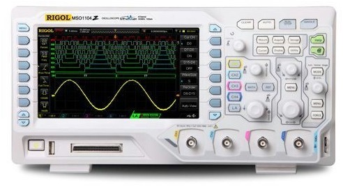
The newest generation of scopes are MixedSignal Oscilloscopes (MSO), allowing some number of analog input signals, as well as a larger number of digital input signals. An analog signal can have a range of values and we are interested in seeing the actual amplitude of the signal. A digital scope must store the n bits from the ADC for each sample. A digital signal has two values, true or false. Like any other digital device, these truth values are mapped onto voltage thresholds (VH and VL). When the analog voltage, Vin >= VH, then the signal represents true, and when the voltage Vin <= VL, the signal represents false. An MSO scope can digitize the signal and store only the 1’s and 0’s for each sample. As a result, we lose the exact voltage level of the signal, but gain a much wider input bus. For example, many MSO scopes have 2 or 4 analog inputs, but have 16 (or more) digital inputs. When using the analog inputs, an MSO scope is equivalent to a DSO.
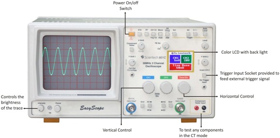
Essential Parts and Controls of Digital Storage Oscilloscope
Almost every oscilloscope will have the following parts / controls:
Display The display on the oscilloscope shows the current status of the signal
Graticule The display has a horizontal and vertical lines dividing the screen into a grid. In the Yaxis, each horizontal line represents some number of Volts / Division.Along the Xaxis, each vertical line represents the number of Seconds / Division. The graticule helps reference the value of the signal. Controls on the scope can change the Volts/Div and the Seconds/Div for the captured signal. The term graticule is a hold over from the days of CRT tubes when the lines would be physically etched on the CRT display.
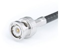 Analog Input Channels The input channels are located on the front of the unit. The input channels are the industry standard Bayonet NeillConcelman (BNC) connectors. The inner conductor carries the signal, and the outer shielding connects common ground. It is important to always have the oscilloscope connected to ground.
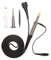 Analog Probes The scopes probes have a BNC connection on one end, and both ground and probe tip on the other end. Probes can be connected to any of the input channels on the front of the scope. The analog probes can be connected to any of the analog input channels. This allows different parts of a circuit to be simultaneously captured and analyzed.
Horizontal Scale Controls This knob on the oscilloscope adjusts the time per division. Turning the horizontal knob to the counterclockwise increases the time per division, and clockwise decreases the timer per division. The absolute minimum and maximum are determined by the properties of the oscilloscope. Generally, as the horizontal scale decreases more of the instantaneous details of the signal are visible but then less of the signal’s period will be visible. If the scope has 12 horizontal graticules, and the timebase is set for 1ms / division, then 12ms of the signal will be displayed at a given time.
Vertical Scale Controls The vertical scale on the scope adjusts the volts per division. Turning the knob counterclockwise increases the volts per division, and clockwise decreases it. As the voltage decreases, less peaktopeak amplitude will be visible, but the signal will also show increased sensitivity (smaller changes to amplitude). If the scope has 8 vertical graticules and the voltagescale is set for 1V / division, then 8V of amplitude (peaktopeak) can be displayed, which could be 4V to 4V, or 0 to 8V, or even 5V to 13V.
Horizontal Position Control This knob will change the displayed horizontal position. The scope captures more data that can be displayed on a screen. Change the horizontal position will allow different parts of the signal to be displayed
Vertical Position Control This knob will translate the drawn signal up and down on the screen. This is especially useful when there are multiple channels active or when the voltage has a DC bias. For example, if the capture signal has a peaktopeak amplitude of 5V to 13V, using the vertical control could bring the “top” of the signal down to the center of the screen, allowing a fullrange of display.
Trigger Control Most oscilloscopes have one or more different triggers. The trigger controls allow the selection and configuration of the trigger and the associated display options. For example, a common trigger mode is called edge triggering which can detect when a signal crosses a threshold. When this happens, the scope will display signal right before and right after the event.
Vernier Dials These allows the knob to have dual functionality. Pressing in and turning the knob will have different behavior than simply turning it. For example, the vertical scale makes small adjustments (.1V/div) unless it is pressed in, then the adjustments are much larger.
Select your DSO based on Performance Terms
Oscilloscopes have several key performance characteristics. These determine what types of signals can be captured by the scope and the associated probes.
Bandwidth Bandwidth describes the frequency range of the oscilloscope (in Megahertz MHz). The bandwidth describes the frequency at which the sampled signal’s amplitude will be attenuated to 70.7% of its original value (that is 3 dB attenuation in signals terms). Signal attenuation describes a reduction in the strength of a signal during transmission. Thus, a signal that was transmitted with 1V peaktopeak amplitude at 100MHz would be received at 0.7V peaktopeak amplitude on a 100MHz scope.
The figure below shows a typical attenuation curve. As the frequency goes up, attenuation losses mount and error rates increase. To measure a signal with 3% loss, we are limited to 30% of the scope’s bandwidth.
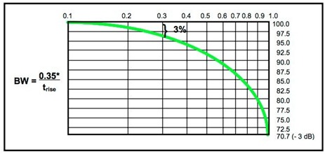
As the signal degrades, it will have the same general shape, it would be considerably degraded and not useful for serious analysis. Smaller perturbations in the input signal will be lost entirely. Also note that the steepness of the curve suggests that exceeding the upper-bandwidth limit may yield a captured signal, it will be of very poor quality.
Most vendors recommend the 5times rule: select an oscilloscope that has 5times the bandwidth as the fastest signal to be measured. To accurately capture a signal at 100MHz would require a 500MHz scope.
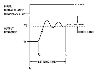
Risetime Parasitic induction and other factors can cause highfrequency noise when a signal makes an edge transition. If the scope’s risetime is slower than the signal’s rise time, the scope will show a “falsepositive” signal that may actually cause the deviceundertest (DUT) to reject. There is another 5times rule, such that the scope’s risetime should be 5times faster than the fastest signal.
Sample Rate Digital scopes must convert an analog value into a digital sample and store that in the scope’s memory. The stored signal is then visually reconstructed on the display with missing data interpolated as if the data were actually present. Interpolated data is not actually present, rather it is simply made up mathematically. The higher the sampling rate, the more samples are recorded, and the fewer points are interpolated, and the more faithful the signal will be to its original. The Nyquist theorem requires at least 2times the number of samples per second as the highest frequency to have reasonable reconstruction, but that is a minimum.
Oversampling captures more points and provides a more accurate display. The recommendation is another 5times rule: the scope’s sampling rate should be at least 5 times than the fastest frequency.
Example: a 100MHz sampled signal needs at least 500M samps/sec (on a 500MHz scope).
Record Length / Memory Size Digital scopes store the captured data into memory. The larger the memory the greater the record length, the more time a signal can be captured. The time is:
Tacq = record length / sample rate
Having a larger record length allows a digital scope to allow the user to scroll through more than one screenful of data, or to perform more advanced analysis and triggering. With more memory, the same signal can be captured with a higher sample rate to enable a more accurate reconstruction.


 combined with superior switching performance")


